DTensor 101: Mesh, Layout, and SPMD in TensorFlow

Content Overview

• Overview
• Setup
• DTensor’s model of distributed tensors
• Mesh
• Layout
• Single-client and multi-client applications
• DTensor as a sharded tensor
• Anatomy of a DTensor
• Sharding a DTensor to a Mesh
• TensorFlow API on DTensor
• DTensor as operands
• DTensor as output
• From tf.Variable to dtensor.DVariable
• What’s next?

\ \

Overview

This colab introduces DTensor, an extension to TensorFlow for synchronous distributed computing.

DTensor provides a global programming model that allows developers to compose applications that operate on Tensors globally while managing the distribution across devices internally. DTensor distributes the program and tensors according to the sharding directives through a procedure called Single program, multiple data (SPMD) expansion.

By decoupling the application from sharding directives, DTensor enables running the same application on a single device, multiple devices, or even multiple clients, while preserving its global semantics.

This guide introduces DTensor concepts for distributed computing, and how DTensor integrates with TensorFlow. For a demo of using DTensor in model training, refer to the Distributed training with DTensor tutorial.

Setup

DTensor (tf.experimental.dtensor) has been part of TensorFlow since the 2.9.0 release.

Begin by importing TensorFlow, dtensor, and configure TensorFlow to use 6 virtual CPUs. Even though this example uses virtual CPUs, DTensor works the same way on CPU, GPU or TPU devices.

\

import tensorflow as tf from tensorflow.experimental import dtensor  print('TensorFlow version:', tf.__version__)  def configure_virtual_cpus(ncpu):   phy_devices = tf.config.list_physical_devices('CPU')   tf.config.set_logical_device_configuration(phy_devices[0], [         tf.config.LogicalDeviceConfiguration(),     ] * ncpu)  configure_virtual_cpus(6) DEVICES = [f'CPU:{i}' for i in range(6)]  tf.config.list_logical_devices('CPU') 

\

2024-08-15 03:07:05.476728: E external/local_xla/xla/stream_executor/cuda/cuda_fft.cc:485] Unable to register cuFFT factory: Attempting to register factory for plugin cuFFT when one has already been registered 2024-08-15 03:07:05.497944: E external/local_xla/xla/stream_executor/cuda/cuda_dnn.cc:8454] Unable to register cuDNN factory: Attempting to register factory for plugin cuDNN when one has already been registered 2024-08-15 03:07:05.504401: E external/local_xla/xla/stream_executor/cuda/cuda_blas.cc:1452] Unable to register cuBLAS factory: Attempting to register factory for plugin cuBLAS when one has already been registered TensorFlow version: 2.17.0 WARNING: All log messages before absl::InitializeLog() is called are written to STDERR I0000 00:00:1723691228.106716  179173 cuda_executor.cc:1015] successful NUMA node read from SysFS had negative value (-1), but there must be at least one NUMA node, so returning NUMA node zero. See more at https://github.com/torvalds/linux/blob/v6.0/Documentation/ABI/testing/sysfs-bus-pci#L344-L355 I0000 00:00:1723691228.110575  179173 cuda_executor.cc:1015] successful NUMA node read from SysFS had negative value (-1), but there must be at least one NUMA node, so returning NUMA node zero. See more at https://github.com/torvalds/linux/blob/v6.0/Documentation/ABI/testing/sysfs-bus-pci#L344-L355 I0000 00:00:1723691228.114281  179173 cuda_executor.cc:1015] successful NUMA node read from SysFS had negative value (-1), but there must be at least one NUMA node, so returning NUMA node zero. See more at https://github.com/torvalds/linux/blob/v6.0/Documentation/ABI/testing/sysfs-bus-pci#L344-L355 I0000 00:00:1723691228.117515  179173 cuda_executor.cc:1015] successful NUMA node read from SysFS had negative value (-1), but there must be at least one NUMA node, so returning NUMA node zero. See more at https://github.com/torvalds/linux/blob/v6.0/Documentation/ABI/testing/sysfs-bus-pci#L344-L355 I0000 00:00:1723691228.129071  179173 cuda_executor.cc:1015] successful NUMA node read from SysFS had negative value (-1), but there must be at least one NUMA node, so returning NUMA node zero. See more at https://github.com/torvalds/linux/blob/v6.0/Documentation/ABI/testing/sysfs-bus-pci#L344-L355 I0000 00:00:1723691228.132633  179173 cuda_executor.cc:1015] successful NUMA node read from SysFS had negative value (-1), but there must be at least one NUMA node, so returning NUMA node zero. See more at https://github.com/torvalds/linux/blob/v6.0/Documentation/ABI/testing/sysfs-bus-pci#L344-L355 I0000 00:00:1723691228.136108  179173 cuda_executor.cc:1015] successful NUMA node read from SysFS had negative value (-1), but there must be at least one NUMA node, so returning NUMA node zero. See more at https://github.com/torvalds/linux/blob/v6.0/Documentation/ABI/testing/sysfs-bus-pci#L344-L355 I0000 00:00:1723691228.139126  179173 cuda_executor.cc:1015] successful NUMA node read from SysFS had negative value (-1), but there must be at least one NUMA node, so returning NUMA node zero. See more at https://github.com/torvalds/linux/blob/v6.0/Documentation/ABI/testing/sysfs-bus-pci#L344-L355 I0000 00:00:1723691228.142544  179173 cuda_executor.cc:1015] successful NUMA node read from SysFS had negative value (-1), but there must be at least one NUMA node, so returning NUMA node zero. See more at https://github.com/torvalds/linux/blob/v6.0/Documentation/ABI/testing/sysfs-bus-pci#L344-L355 I0000 00:00:1723691228.145949  179173 cuda_executor.cc:1015] successful NUMA node read from SysFS had negative value (-1), but there must be at least one NUMA node, so returning NUMA node zero. See more at https://github.com/torvalds/linux/blob/v6.0/Documentation/ABI/testing/sysfs-bus-pci#L344-L355 I0000 00:00:1723691228.149337  179173 cuda_executor.cc:1015] successful NUMA node read from SysFS had negative value (-1), but there must be at least one NUMA node, so returning NUMA node zero. See more at https://github.com/torvalds/linux/blob/v6.0/Documentation/ABI/testing/sysfs-bus-pci#L344-L355 I0000 00:00:1723691228.152299  179173 cuda_executor.cc:1015] successful NUMA node read from SysFS had negative value (-1), but there must be at least one NUMA node, so returning NUMA node zero. See more at https://github.com/torvalds/linux/blob/v6.0/Documentation/ABI/testing/sysfs-bus-pci#L344-L355 I0000 00:00:1723691229.367903  179173 cuda_executor.cc:1015] successful NUMA node read from SysFS had negative value (-1), but there must be at least one NUMA node, so returning NUMA node zero. See more at https://github.com/torvalds/linux/blob/v6.0/Documentation/ABI/testing/sysfs-bus-pci#L344-L355 I0000 00:00:1723691229.370038  179173 cuda_executor.cc:1015] successful NUMA node read from SysFS had negative value (-1), but there must be at least one NUMA node, so returning NUMA node zero. See more at https://github.com/torvalds/linux/blob/v6.0/Documentation/ABI/testing/sysfs-bus-pci#L344-L355 I0000 00:00:1723691229.372091  179173 cuda_executor.cc:1015] successful NUMA node read from SysFS had negative value (-1), but there must be at least one NUMA node, so returning NUMA node zero. See more at https://github.com/torvalds/linux/blob/v6.0/Documentation/ABI/testing/sysfs-bus-pci#L344-L355 I0000 00:00:1723691229.374176  179173 cuda_executor.cc:1015] successful NUMA node read from SysFS had negative value (-1), but there must be at least one NUMA node, so returning NUMA node zero. See more at https://github.com/torvalds/linux/blob/v6.0/Documentation/ABI/testing/sysfs-bus-pci#L344-L355 I0000 00:00:1723691229.376222  179173 cuda_executor.cc:1015] successful NUMA node read from SysFS had negative value (-1), but there must be at least one NUMA node, so returning NUMA node zero. See more at https://github.com/torvalds/linux/blob/v6.0/Documentation/ABI/testing/sysfs-bus-pci#L344-L355 I0000 00:00:1723691229.378197  179173 cuda_executor.cc:1015] successful NUMA node read from SysFS had negative value (-1), but there must be at least one NUMA node, so returning NUMA node zero. See mo [LogicalDevice(name='/device:CPU:0', device_type='CPU'),  LogicalDevice(name='/device:CPU:1', device_type='CPU'),  LogicalDevice(name='/device:CPU:2', device_type='CPU'),  LogicalDevice(name='/device:CPU:3', device_type='CPU'),  LogicalDevice(name='/device:CPU:4', device_type='CPU'),  LogicalDevice(name='/device:CPU:5', device_type='CPU')] re at https://github.com/torvalds/linux/blob/v6.0/Documentation/ABI/testing/sysfs-bus-pci#L344-L355 I0000 00:00:1723691229.380105  179173 cuda_executor.cc:1015] successful NUMA node read from SysFS had negative value (-1), but there must be at least one NUMA node, so returning NUMA node zero. See more at https://github.com/torvalds/linux/blob/v6.0/Documentation/ABI/testing/sysfs-bus-pci#L344-L355 I0000 00:00:1723691229.382049  179173 cuda_executor.cc:1015] successful NUMA node read from SysFS had negative value (-1), but there must be at least one NUMA node, so returning NUMA node zero. See more at https://github.com/torvalds/linux/blob/v6.0/Documentation/ABI/testing/sysfs-bus-pci#L344-L355 I0000 00:00:1723691229.383990  179173 cuda_executor.cc:1015] successful NUMA node read from SysFS had negative value (-1), but there must be at least one NUMA node, so returning NUMA node zero. See more at https://github.com/torvalds/linux/blob/v6.0/Documentation/ABI/testing/sysfs-bus-pci#L344-L355 I0000 00:00:1723691229.385954  179173 cuda_executor.cc:1015] successful NUMA node read from SysFS had negative value (-1), but there must be at least one NUMA node, so returning NUMA node zero. See more at https://github.com/torvalds/linux/blob/v6.0/Documentation/ABI/testing/sysfs-bus-pci#L344-L355 I0000 00:00:1723691229.387849  179173 cuda_executor.cc:1015] successful NUMA node read from SysFS had negative value (-1), but there must be at least one NUMA node, so returning NUMA node zero. See more at https://github.com/torvalds/linux/blob/v6.0/Documentation/ABI/testing/sysfs-bus-pci#L344-L355 I0000 00:00:1723691229.389820  179173 cuda_executor.cc:1015] successful NUMA node read from SysFS had negative value (-1), but there must be at least one NUMA node, so returning NUMA node zero. See more at https://github.com/torvalds/linux/blob/v6.0/Documentation/ABI/testing/sysfs-bus-pci#L344-L355 I0000 00:00:1723691229.428143  179173 cuda_executor.cc:1015] successful NUMA node read from SysFS had negative value (-1), but there must be at least one NUMA node, so returning NUMA node zero. See more at https://github.com/torvalds/linux/blob/v6.0/Documentation/ABI/testing/sysfs-bus-pci#L344-L355 I0000 00:00:1723691229.430312  179173 cuda_executor.cc:1015] successful NUMA node read from SysFS had negative value (-1), but there must be at least one NUMA node, so returning NUMA node zero. See more at https://github.com/torvalds/linux/blob/v6.0/Documentation/ABI/testing/sysfs-bus-pci#L344-L355 I0000 00:00:1723691229.432260  179173 cuda_executor.cc:1015] successful NUMA node read from SysFS had negative value (-1), but there must be at least one NUMA node, so returning NUMA node zero. See more at https://github.com/torvalds/linux/blob/v6.0/Documentation/ABI/testing/sysfs-bus-pci#L344-L355 I0000 00:00:1723691229.434249  179173 cuda_executor.cc:1015] successful NUMA node read from SysFS had negative value (-1), but there must be at least one NUMA node, so returning NUMA node zero. See more at https://github.com/torvalds/linux/blob/v6.0/Documentation/ABI/testing/sysfs-bus-pci#L344-L355 I0000 00:00:1723691229.436210  179173 cuda_executor.cc:1015] successful NUMA node read from SysFS had negative value (-1), but there must be at least one NUMA node, so returning NUMA node zero. See more at https://github.com/torvalds/linux/blob/v6.0/Documentation/ABI/testing/sysfs-bus-pci#L344-L355 I0000 00:00:1723691229.438213  179173 cuda_executor.cc:1015] successful NUMA node read from SysFS had negative value (-1), but there must be at least one NUMA node, so returning NUMA node zero. See more at https://github.com/torvalds/linux/blob/v6.0/Documentation/ABI/testing/sysfs-bus-pci#L344-L355 I0000 00:00:1723691229.440127  179173 cuda_executor.cc:1015] successful NUMA node read from SysFS had negative value (-1), but there must be at least one NUMA node, so returning NUMA node zero. See more at https://github.com/torvalds/linux/blob/v6.0/Documentation/ABI/testing/sysfs-bus-pci#L344-L355 I0000 00:00:1723691229.442098  179173 cuda_executor.cc:1015] successful NUMA node read from SysFS had negative value (-1), but there must be at least one NUMA node, so returning NUMA node zero. See more at https://github.com/torvalds/linux/blob/v6.0/Documentation/ABI/testing/sysfs-bus-pci#L344-L355 I0000 00:00:1723691229.444069  179173 cuda_executor.cc:1015] successful NUMA node read from SysFS had negative value (-1), but there must be at least one NUMA node, so returning NUMA node zero. See more at https://github.com/torvalds/linux/blob/v6.0/Documentation/ABI/testing/sysfs-bus-pci#L344-L355 I0000 00:00:1723691229.446542  179173 cuda_executor.cc:1015] successful NUMA node read from SysFS had negative value (-1), but there must be at least one NUMA node, so returning NUMA node zero. See more at https://github.com/torvalds/linux/blob/v6.0/Documentation/ABI/testing/sysfs-bus-pci#L344-L355 I0000 00:00:1723691229.448849  179173 cuda_executor.cc:1015] successful NUMA node read from SysFS had negative value (-1), but there must be at least one NUMA node, so returning NUMA node zero. See more at https://github.com/torvalds/linux/blob/v6.0/Documentation/ABI/testing/sysfs-bus-pci#L344-L355 I0000 00:00:1723691229.451234  179173 cuda_executor.cc:1015] successful NUMA node read from SysFS had negative value (-1), but there must be at least one NUMA node, so returning NUMA node zero. See more at https://github.com/torvalds/linux/blob/v6.0/Documentation/ABI/testing/sysfs-bus-pci#L344-L355 

DTensor's model of distributed tensors

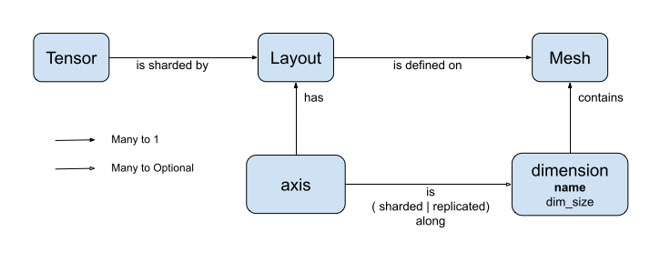
DTensor introduces two concepts: dtensor.Mesh and dtensor.Layout. They are abstractions to model the sharding of tensors across topologically related devices.

• Mesh defines the device list for computation.
• Layout defines how to shard the Tensor dimension on a Mesh.

Mesh

Mesh represents a logical Cartisian topology of a set of devices. Each dimension of the Cartisian grid is called a Mesh dimension, and referred to with a name. Names of mesh dimension within the same Mesh must be unique.

Names of mesh dimensions are referenced by Layout to describe the sharding behavior of a tf.Tensor along each of its axes. This is described in more detail later in the section on Layout.

Mesh can be thought of as a multi-dimensional array of devices.

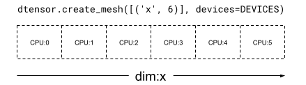
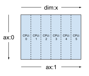
In a 1 dimensional Mesh, all devices form a list in a single mesh dimension. The following example uses dtensor.create_mesh to create a mesh from 6 CPU devices along a mesh dimension 'x' with a size of 6 devices:

\

mesh_1d = dtensor.create_mesh([('x', 6)], devices=DEVICES) print(mesh_1d) 

\

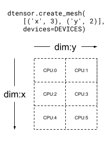
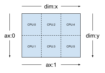
Mesh.from_string(|x=6|0,1,2,3,4,5|0,1,2,3,4,5|/job:localhost/replica:0/task:0/device:CPU:0,/job:localhost/replica:0/task:0/device:CPU:1,/job:localhost/replica:0/task:0/device:CPU:2,/job:localhost/replica:0/task:0/device:CPU:3,/job:localhost/replica:0/task:0/device:CPU:4,/job:localhost/replica:0/task:0/device:CPU:5) 

A Mesh can be multi dimensional as well. In the following example, 6 CPU devices form a 3x2 mesh, where the 'x' mesh dimension has a size of 3 devices, and the 'y' mesh dimension has a size of 2 devices:

\

mesh_2d = dtensor.create_mesh([('x', 3), ('y', 2)], devices=DEVICES) print(mesh_2d) 

\

Mesh.from_string(|x=3,y=2|0,1,2,3,4,5|0,1,2,3,4,5|/job:localhost/replica:0/task:0/device:CPU:0,/job:localhost/replica:0/task:0/device:CPU:1,/job:localhost/replica:0/task:0/device:CPU:2,/job:localhost/replica:0/task:0/device:CPU:3,/job:localhost/replica:0/task:0/device:CPU:4,/job:localhost/replica:0/task:0/device:CPU:5) 

Layout

Layout specifies how a tensor is distributed, or sharded, on a Mesh.

\

:::tip Note: In order to avoid confusions between Mesh and Layout, the term dimension is always associated with Mesh, and the term axis with Tensor and Layout in this guide.

:::

The rank of Layout should be the same as the rank of the Tensor where the Layout is applied. For each of the Tensor's axes the Layout may specify a mesh dimension to shard the tensor across, or specify the axis as "unsharded". The tensor is replicated across any mesh dimensions that it is not sharded across.

The rank of a Layout and the number of dimensions of a Mesh do not need to match. The unsharded axes of a Layout do not need to be associated to a mesh dimension, and unsharded mesh dimensions do not need to be associated with a layout axis.

Let's analyze a few examples of Layout for the Mesh's created in the previous section.

On a 1-dimensional mesh such as [("x", 6)] (mesh_1d in the previous section), Layout(["unsharded", "unsharded"], mesh_1d) is a layout for a rank-2 tensor replicated across 6 devices.

\

layout = dtensor.Layout([dtensor.UNSHARDED, dtensor.UNSHARDED], mesh_1d) 

Using the same tensor and mesh the layout Layout(['unsharded', 'x']) would shard the second axis of the tensor across the 6 devices.

\

layout = dtensor.Layout([dtensor.UNSHARDED, 'x'], mesh_1d) 

Given a 2-dimensional 3x2 mesh such as [("x", 3), ("y", 2)], (mesh_2d from the previous section), Layout(["y", "x"], mesh_2d) is a layout for a rank-2 Tensor whose first axis is sharded across mesh dimension "y", and whose second axis is sharded across mesh dimension "x".

\

\

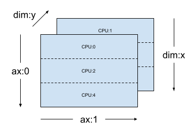
layout = dtensor.Layout(['y', 'x'], mesh_2d) 

For the same mesh_2d, the layout Layout(["x", dtensor.UNSHARDED], mesh_2d) is a layout for a rank-2 Tensor that is replicated across "y", and whose first axis is sharded on mesh dimension x.

\

layout = dtensor.Layout(["x", dtensor.UNSHARDED], mesh_2d) 

Single-client and multi-client applications

DTensor supports both single-client and multi-client applications. The colab Python kernel is an example of a single client DTensor application, where there is a single Python process.

In a multi-client DTensor application, multiple Python processes collectively perform as a coherent application. The Cartisian grid of a Mesh in a multi-client DTensor application can span across devices regardless of whether they are attached locally to the current client or attached remotely to another client. The set of all devices used by a Mesh are called the global device list.

The creation of a Mesh in a multi-client DTensor application is a collective operation where the global device list is identical for all of the participating clients, and the creation of the Mesh serves as a global barrier.

During Mesh creation, each client provides its local device list together with the expected global device list. DTensor validates that both lists are consistent. Please refer to the API documentation for dtensor.create_mesh and dtensor.create_distributed_mesh for more information on multi-client mesh creation and the global device list.

Single-client can be thought of as a special case of multi-client, with 1 client. In a single-client application, the global device list is identical to the local device list.

DTensor as a sharded tensor

Now, start coding with DTensor. The helper function, dtensor_from_array, demonstrates creating DTensors from something that looks like a tf.Tensor. The function performs two steps:

• Replicates the tensor to every device on the mesh.
• Shards the copy according to the layout requested in its arguments.

\

def dtensor_from_array(arr, layout, shape=None, dtype=None):   """Convert a DTensor from something that looks like an array or Tensor.    This function is convenient for quick doodling DTensors from a known,   unsharded data object in a single-client environment. This is not the   most efficient way of creating a DTensor, but it will do for this   tutorial.   """   if shape is not None or dtype is not None:     arr = tf.constant(arr, shape=shape, dtype=dtype)    # replicate the input to the mesh   a = dtensor.copy_to_mesh(arr,           layout=dtensor.Layout.replicated(layout.mesh, rank=layout.rank))   # shard the copy to the desirable layout   return dtensor.relayout(a, layout=layout) 

Anatomy of a DTensor

A DTensor is a tf.Tensor object, but augumented with the Layout annotation that defines its sharding behavior. A DTensor consists of the following:

• Global tensor meta-data, including the global shape and dtype of the tensor.
• A Layout, which defines the Mesh the Tensor belongs to, and how the Tensor is sharded onto the Mesh.
• A list of component tensors, one item per local device in the Mesh.

With dtensor_from_array, you can create your first DTensor, my_first_dtensor, and examine its contents:

\

mesh = dtensor.create_mesh([("x", 6)], devices=DEVICES) layout = dtensor.Layout([dtensor.UNSHARDED], mesh)  my_first_dtensor = dtensor_from_array([0, 1], layout)  # Examine the DTensor content print(my_first_dtensor) print("global shape:", my_first_dtensor.shape) print("dtype:", my_first_dtensor.dtype) 

\

tf.Tensor([0 1], layout="sharding_specs:unsharded, mesh:|x=6|0,1,2,3,4,5|0,1,2,3,4,5|/job:localhost/replica:0/task:0/device:CPU:0,/job:localhost/replica:0/task:0/device:CPU:1,/job:localhost/replica:0/task:0/device:CPU:2,/job:localhost/replica:0/task:0/device:CPU:3,/job:localhost/replica:0/task:0/device:CPU:4,/job:localhost/replica:0/task:0/device:CPU:5", shape=(2,), dtype=int32) global shape: (2,) dtype: <dtype: 'int32'> 

Layout and fetch_layout

The layout of a DTensor is not a regular attribute of tf.Tensor. Instead, DTensor provides a function, dtensor.fetch_layout to access the layout of a DTensor:

\

print(dtensor.fetch_layout(my_first_dtensor)) assert layout == dtensor.fetch_layout(my_first_dtensor) 

\

Layout.from_string(sharding_specs:unsharded, mesh:|x=6|0,1,2,3,4,5|0,1,2,3,4,5|/job:localhost/replica:0/task:0/device:CPU:0,/job:localhost/replica:0/task:0/device:CPU:1,/job:localhost/replica:0/task:0/device:CPU:2,/job:localhost/replica:0/task:0/device:CPU:3,/job:localhost/replica:0/task:0/device:CPU:4,/job:localhost/replica:0/task:0/device:CPU:5) 

Component tensors, pack and unpack

A DTensor consists of a list of component tensors. The component tensor for a device in the Mesh is the Tensor object representing the piece of the global DTensor that is stored on this device.

A DTensor can be unpacked into component tensors through dtensor.unpack. You can make use of dtensor.unpack to inspect the components of the DTensor, and confirm they are on all devices of the Mesh.

Note that the positions of component tensors in the global view may overlap each other. For example, in the case of a fully replicated layout, all components are identical replicas of the global tensor.

\

for component_tensor in dtensor.unpack(my_first_dtensor):   print("Device:", component_tensor.device, ",", component_tensor) 

\

Device: /job:localhost/replica:0/task:0/device:CPU:0 , tf.Tensor([0 1], shape=(2,), dtype=int32) Device: /job:localhost/replica:0/task:0/device:CPU:1 , tf.Tensor([0 1], shape=(2,), dtype=int32) Device: /job:localhost/replica:0/task:0/device:CPU:2 , tf.Tensor([0 1], shape=(2,), dtype=int32) Device: /job:localhost/replica:0/task:0/device:CPU:3 , tf.Tensor([0 1], shape=(2,), dtype=int32) Device: /job:localhost/replica:0/task:0/device:CPU:4 , tf.Tensor([0 1], shape=(2,), dtype=int32) Device: /job:localhost/replica:0/task:0/device:CPU:5 , tf.Tensor([0 1], shape=(2,), dtype=int32) 

As shown, my_first_dtensor is a tensor of [0, 1] replicated to all 6 devices.

The inverse operation of dtensor.unpack is dtensor.pack. Component tensors can be packed back into a DTensor.

The components must have the same rank and dtype, which will be the rank and dtype of the returned DTensor. However, there is no strict requirement on the device placement of component tensors as inputs of dtensor.unpack: the function will automatically copy the component tensors to their respective corresponding devices.

\

packed_dtensor = dtensor.pack(     [[0, 1], [0, 1], [0, 1],      [0, 1], [0, 1], [0, 1]],      layout=layout ) print(packed_dtensor) 

\

tf.Tensor([0 1], layout="sharding_specs:unsharded, mesh:|x=6|0,1,2,3,4,5|0,1,2,3,4,5|/job:localhost/replica:0/task:0/device:CPU:0,/job:localhost/replica:0/task:0/device:CPU:1,/job:localhost/replica:0/task:0/device:CPU:2,/job:localhost/replica:0/task:0/device:CPU:3,/job:localhost/replica:0/task:0/device:CPU:4,/job:localhost/replica:0/task:0/device:CPU:5", shape=(2,), dtype=int32) 

Sharding a DTensor to a Mesh

So far you've worked with the my_first_dtensor, which is a rank-1 DTensor fully replicated across a dim-1 Mesh.

Next, create and inspect DTensors that are sharded across a dim-2 Mesh. The following example does this with a 3x2 Mesh on 6 CPU devices, where size of mesh dimension 'x' is 3 devices, and size of mesh dimension'y' is 2 devices:

\

mesh = dtensor.create_mesh([("x", 3), ("y", 2)], devices=DEVICES) 

Fully sharded rank-2 Tensor on a dim-2 Mesh

Create a 3x2 rank-2 DTensor, sharding its first axis along the 'x' mesh dimension, and its second axis along the 'y' mesh dimension.

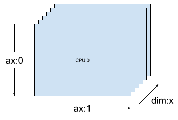
• Because the tensor shape equals to the mesh dimension along all of the sharded axes, each device receives a single element of the DTensor.
• The rank of the component tensor is always the same as the rank of the global shape. DTensor adopts this convention as a simple way to preserve information for locating the relation between a component tensor and the global DTensor.

\

fully_sharded_dtensor = dtensor_from_array(     tf.reshape(tf.range(6), (3, 2)),     layout=dtensor.Layout(["x", "y"], mesh))  for raw_component in dtensor.unpack(fully_sharded_dtensor):   print("Device:", raw_component.device, ",", raw_component) 

\

Device: /job:localhost/replica:0/task:0/device:CPU:0 , tf.Tensor([[0]], shape=(1, 1), dtype=int32) Device: /job:localhost/replica:0/task:0/device:CPU:1 , tf.Tensor([[1]], shape=(1, 1), dtype=int32) Device: /job:localhost/replica:0/task:0/device:CPU:2 , tf.Tensor([[2]], shape=(1, 1), dtype=int32) Device: /job:localhost/replica:0/task:0/device:CPU:3 , tf.Tensor([[3]], shape=(1, 1), dtype=int32) Device: /job:localhost/replica:0/task:0/device:CPU:4 , tf.Tensor([[4]], shape=(1, 1), dtype=int32) Device: /job:localhost/replica:0/task:0/device:CPU:5 , tf.Tensor([[5]], shape=(1, 1), dtype=int32) 

Fully replicated rank-2 Tensor on a dim-2 Mesh

For comparison, create a 3x2 rank-2 DTensor, fully replicated to the same dim-2 Mesh.

• Because the DTensor is fully replicated, each device receives a full replica of the 3x2 DTensor.
• The rank of the component tensors are the same as the rank of the global shape -- this fact is trivial, because in this case, the shape of the component tensors are the same as the global shape anyway.

\

fully_replicated_dtensor = dtensor_from_array(     tf.reshape(tf.range(6), (3, 2)),     layout=dtensor.Layout([dtensor.UNSHARDED, dtensor.UNSHARDED], mesh)) # Or, layout=tensor.Layout.fully_replicated(mesh, rank=2)  for component_tensor in dtensor.unpack(fully_replicated_dtensor):   print("Device:", component_tensor.device, ",", component_tensor) 

\

Device: /job:localhost/replica:0/task:0/device:CPU:0 , tf.Tensor( [[0 1]  [2 3]  [4 5]], shape=(3, 2), dtype=int32) Device: /job:localhost/replica:0/task:0/device:CPU:1 , tf.Tensor( [[0 1]  [2 3]  [4 5]], shape=(3, 2), dtype=int32) Device: /job:localhost/replica:0/task:0/device:CPU:2 , tf.Tensor( [[0 1]  [2 3]  [4 5]], shape=(3, 2), dtype=int32) Device: /job:localhost/replica:0/task:0/device:CPU:3 , tf.Tensor( [[0 1]  [2 3]  [4 5]], shape=(3, 2), dtype=int32) Device: /job:localhost/replica:0/task:0/device:CPU:4 , tf.Tensor( [[0 1]  [2 3]  [4 5]], shape=(3, 2), dtype=int32) Device: /job:localhost/replica:0/task:0/device:CPU:5 , tf.Tensor( [[0 1]  [2 3]  [4 5]], shape=(3, 2), dtype=int32) 

Hybrid rank-2 Tensor on a dim-2 Mesh

What about somewhere between fully sharded and fully replicated?

DTensor allows a Layout to be a hybrid, sharded along some axes, but replicated along others.

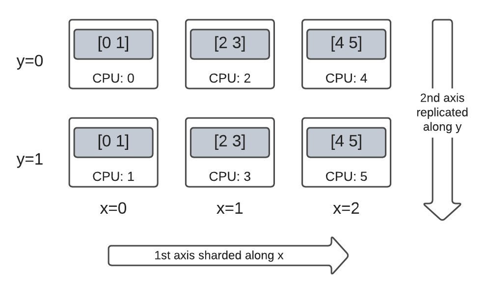
For example, you can shard the same 3x2 rank-2 DTensor in the following way:

• 1st axis sharded along the 'x' mesh dimension.
• 2nd axis replicated along the 'y' mesh dimension.

To achieve this sharding scheme, you just need to replace the sharding spec of the 2nd axis from 'y' to dtensor.UNSHARDED, to indicate your intention of replicating along the 2nd axis. The layout object will look like Layout(['x', dtensor.UNSHARDED], mesh):

\

hybrid_sharded_dtensor = dtensor_from_array(     tf.reshape(tf.range(6), (3, 2)),     layout=dtensor.Layout(['x', dtensor.UNSHARDED], mesh))  for component_tensor in dtensor.unpack(hybrid_sharded_dtensor):   print("Device:", component_tensor.device, ",", component_tensor) 

\

Device: /job:localhost/replica:0/task:0/device:CPU:0 , tf.Tensor([[0 1]], shape=(1, 2), dtype=int32) Device: /job:localhost/replica:0/task:0/device:CPU:1 , tf.Tensor([[0 1]], shape=(1, 2), dtype=int32) Device: /job:localhost/replica:0/task:0/device:CPU:2 , tf.Tensor([[2 3]], shape=(1, 2), dtype=int32) Device: /job:localhost/replica:0/task:0/device:CPU:3 , tf.Tensor([[2 3]], shape=(1, 2), dtype=int32) Device: /job:localhost/replica:0/task:0/device:CPU:4 , tf.Tensor([[4 5]], shape=(1, 2), dtype=int32) Device: /job:localhost/replica:0/task:0/device:CPU:5 , tf.Tensor([[4 5]], shape=(1, 2), dtype=int32) 

You can inspect the component tensors of the created DTensor and verify they are indeed sharded according to your scheme. It may be helpful to illustrate the situation with a chart:

Tensor.numpy() and sharded DTensor

Be aware that calling the .numpy() method on a sharded DTensor raises an error. The rationale for erroring is to protect against unintended gathering of data from multiple computing devices to the host CPU device backing the returned NumPy array:

\

print(fully_replicated_dtensor.numpy())  try:   fully_sharded_dtensor.numpy() except tf.errors.UnimplementedError:   print("got an error as expected for fully_sharded_dtensor")  try:   hybrid_sharded_dtensor.numpy() except tf.errors.UnimplementedError:   print("got an error as expected for hybrid_sharded_dtensor") 

\

[[0 1]  [2 3]  [4 5]] got an error as expected for fully_sharded_dtensor got an error as expected for hybrid_sharded_dtensor 

TensorFlow API on DTensor

DTensor strives to be a drop-in replacement for tensor in your program. The TensorFlow Python API that consume tf.Tensor, such as the Ops library functions, tf.function, tf.GradientTape, also work with DTensor.

To accomplish this, for each TensorFlow Graph, DTensor produces and executes an equivalent SPMD graph in a procedure called SPMD expansion. A few critical steps in DTensor SPMD expansion are:

• Propagating the sharding Layout of DTensor in the TensorFlow graph
• Rewriting TensorFlow Ops on the global DTensor with equivalent TensorFlow Ops on the component tensors, inserting collective and communication Ops when necessary
• Lowering backend neutral TensorFlow Ops to backend specific TensorFlow Ops.

The final result is that DTensor is a drop-in replacement for Tensor.

\

:::tip Note: DTensor is still an experimental API which means you will be exploring and pushing the boundaries and limits of the DTensor programming model.

:::

\ There are 2 ways of triggering DTensor execution:

• DTensor as operands of a Python function, such as tf.matmul(a, b), will run through DTensor if a, b, or both are DTensors.
• Requesting the result of a Python function to be a DTensor, such as dtensor.call_with_layout(tf.ones, layout, shape=(3, 2)), will run through DTensor because we requested the output of tf.ones to be sharded according to a layout.

DTensor as operands

Many TensorFlow API functions take tf.Tensor as their operands, and returns tf.Tensor as their results. For these functions, you can express intention to run a function through DTensor by passing in DTensor as operands. This section uses tf.matmul(a, b) as an example.

Fully replicated input and output

In this case, the DTensors are fully replicated. On each of the devices of the Mesh,

• the component tensor for operand a is [[1, 2, 3], [4, 5, 6]] (2x3)
• the component tensor for operand b is [[6, 5], [4, 3], [2, 1]] (3x2)
• the computation consists of a single MatMul of (2x3, 3x2) -> 2x2,
• the component tensor for result c is [[20, 14], [56,41]] (2x2)

Total number of floating point mul operations is 6 device * 4 result * 3 mul = 72.

\

mesh = dtensor.create_mesh([("x", 6)], devices=DEVICES) layout = dtensor.Layout([dtensor.UNSHARDED, dtensor.UNSHARDED], mesh) a = dtensor_from_array([[1, 2, 3], [4, 5, 6]], layout=layout) b = dtensor_from_array([[6, 5], [4, 3], [2, 1]], layout=layout)  c = tf.matmul(a, b) # runs 6 identical matmuls in parallel on 6 devices  # `c` is a DTensor replicated on all devices (same as `a` and `b`) print('Sharding spec:', dtensor.fetch_layout(c).sharding_specs) print("components:") for component_tensor in dtensor.unpack(c):   print(component_tensor.device, component_tensor.numpy()) 

\

Sharding spec: ['unsharded', 'unsharded'] components: /job:localhost/replica:0/task:0/device:CPU:0 [[20 14]  [56 41]] /job:localhost/replica:0/task:0/device:CPU:1 [[20 14]  [56 41]] /job:localhost/replica:0/task:0/device:CPU:2 [[20 14]  [56 41]] /job:localhost/replica:0/task:0/device:CPU:3 [[20 14]  [56 41]] /job:localhost/replica:0/task:0/device:CPU:4 [[20 14]  [56 41]] /job:localhost/replica:0/task:0/device:CPU:5 [[20 14]  [56 41]] 

Sharding operands along the contracted axis

You can reduce the amount of computation per device by sharding the operands a and b. A popular sharding scheme for tf.matmul is to shard the operands along the axis of the contraction, which means sharding a along the second axis, and b along the first axis.

The global matrix product sharded under this scheme can be performed efficiently, by local matmuls that runs concurrently, followed by a collective reduction to aggregate the local results. This is also the canonical way of implementing a distributed matrix dot product.

Total number of floating point mul operations is 6 devices * 4 result * 1 = 24, a factor of 3 reduction compared to the fully replicated case (72) above. The factor of 3 is due to the sharding along x mesh dimension with a size of 3 devices.

The reduction of the number of operations run sequentially is the main mechansism with which synchronuous model parallelism accelerates training.

\

mesh = dtensor.create_mesh([("x", 3), ("y", 2)], devices=DEVICES) a_layout = dtensor.Layout([dtensor.UNSHARDED, 'x'], mesh) a = dtensor_from_array([[1, 2, 3], [4, 5, 6]], layout=a_layout) b_layout = dtensor.Layout(['x', dtensor.UNSHARDED], mesh) b = dtensor_from_array([[6, 5], [4, 3], [2, 1]], layout=b_layout)  c = tf.matmul(a, b) # `c` is a DTensor replicated on all devices (same as `a` and `b`) print('Sharding spec:', dtensor.fetch_layout(c).sharding_specs) 

\

Sharding spec: ['unsharded', 'unsharded'] 

Additional sharding

You can perform additional sharding on the inputs, and they are appropriately carried over to the results. For example, you can apply additional sharding of operand a along its first axis to the 'y' mesh dimension. The additional sharding will be carried over to the first axis of the result c.

Total number of floating point mul operations is 6 devices * 2 result * 1 = 12, an additional factor of 2 reduction compared to the case (24) above. The factor of 2 is due to the sharding along y mesh dimension with a size of 2 devices.

\

mesh = dtensor.create_mesh([("x", 3), ("y", 2)], devices=DEVICES)  a_layout = dtensor.Layout(['y', 'x'], mesh) a = dtensor_from_array([[1, 2, 3], [4, 5, 6]], layout=a_layout) b_layout = dtensor.Layout(['x', dtensor.UNSHARDED], mesh) b = dtensor_from_array([[6, 5], [4, 3], [2, 1]], layout=b_layout)  c = tf.matmul(a, b) # The sharding of `a` on the first axis is carried to `c' print('Sharding spec:', dtensor.fetch_layout(c).sharding_specs) print("components:") for component_tensor in dtensor.unpack(c):   print(component_tensor.device, component_tensor.numpy()) 

\

Sharding spec: ['y', 'unsharded'] components: /job:localhost/replica:0/task:0/device:CPU:0 [[20 14]] /job:localhost/replica:0/task:0/device:CPU:1 [[56 41]] /job:localhost/replica:0/task:0/device:CPU:2 [[20 14]] /job:localhost/replica:0/task:0/device:CPU:3 [[56 41]] /job:localhost/replica:0/task:0/device:CPU:4 [[20 14]] /job:localhost/replica:0/task:0/device:CPU:5 [[56 41]] 

DTensor as output

What about Python functions that do not take operands, but returns a Tensor result that can be sharded? Examples of such functions are:

• tf.ones, tf.zeros, tf.random.stateless_normal

For these Python functions, DTensor provides dtensor.call_with_layout which eagerly executes a Python function with DTensor, and ensures that the returned Tensor is a DTensor with the requested Layout.

\

help(dtensor.call_with_layout) 

\

Help on function call_with_layout in module tensorflow.dtensor.python.api:  call_with_layout(fn: Callable[..., Any], layout: Optional[tensorflow.dtensor.python.layout.Layout], *args, **kwargs) -> Any     Calls a function in the DTensor device scope if `layout` is not None.      If `layout` is not None, `fn` consumes DTensor(s) as input and produces a     DTensor as output; a DTensor is a tf.Tensor with layout-related attributes.      If `layout` is None, `fn` consumes and produces regular tf.Tensors.      Args:       fn: A supported TF API function such as tf.zeros.       layout: Optional, the layout of the output DTensor.       *args:  Arguments given to `fn`.       **kwargs: Keyword arguments given to `fn`.      Returns:       The return value of `fn` transformed to a DTensor if requested. 

The eagerly executed Python function usually only contain a single non-trivial TensorFlow Op.

To use a Python function that emits multiple TensorFlow Ops with dtensor.call_with_layout, the function should be converted to a tf.function. Calling a tf.function is a single TensorFlow Op. When the tf.function is called, DTensor can perform layout propagation when it analyzes the computing graph of the tf.function, before any of the intermediate tensors are materialized.

APIs that emit a single TensorFlow Op

If a function emits a single TensorFlow Op, you can directly apply dtensor.call_with_layout to the function:

\

help(tf.ones) 

\

Help on function ones in module tensorflow.python.ops.array_ops:  ones(shape, dtype=tf.float32, name=None, layout=None)     Creates a tensor with all elements set to one (1).      See also `tf.ones_like`, `tf.zeros`, `tf.fill`, `tf.eye`.      This operation returns a tensor of type `dtype` with shape `shape` and     all elements set to one.      >>> tf.ones([3, 4], tf.int32)     <tf.Tensor: shape=(3, 4), dtype=int32, numpy=     array([[1, 1, 1, 1],            [1, 1, 1, 1],            [1, 1, 1, 1]], dtype=int32)>      Args:       shape: A `list` of integers, a `tuple` of integers, or a 1-D `Tensor` of         type `int32`.       dtype: Optional DType of an element in the resulting `Tensor`. Default is         `tf.float32`.       name: Optional string. A name for the operation.       layout: Optional, `tf.experimental.dtensor.Layout`. If provided, the result         is a [DTensor](https://www.tensorflow.org/guide/dtensor_overview) with the         provided layout.  Returns:       A `Tensor` with all elements set to one (1). 

\

mesh = dtensor.create_mesh([("x", 3), ("y", 2)], devices=DEVICES) ones = dtensor.call_with_layout(tf.ones, dtensor.Layout(['x', 'y'], mesh), shape=(6, 4)) print(ones) 

\

tf.Tensor({"CPU:0": [[1 1]  [1 1]], "CPU:1": [[1 1]  [1 1]], "CPU:2": [[1 1]  [1 1]], "CPU:3": [[1 1]  [1 1]], "CPU:4": [[1 1]  [1 1]], "CPU:5": [[1 1]  [1 1]]}, layout="sharding_specs:x,y, mesh:|x=3,y=2|0,1,2,3,4,5|0,1,2,3,4,5|/job:localhost/replica:0/task:0/device:CPU:0,/job:localhost/replica:0/task:0/device:CPU:1,/job:localhost/replica:0/task:0/device:CPU:2,/job:localhost/replica:0/task:0/device:CPU:3,/job:localhost/replica:0/task:0/device:CPU:4,/job:localhost/replica:0/task:0/device:CPU:5", shape=(6, 4), dtype=float32) 

APIs that emit multiple TensorFlow Ops

If the API emits multiple TensorFlow Ops, convert the function into a single Op through tf.function. For example, tf.random.stateleess_normal:

\

help(tf.random.stateless_normal) 

\

Help on function stateless_random_normal in module tensorflow.python.ops.stateless_random_ops:  stateless_random_normal(shape, seed, mean=0.0, stddev=1.0, dtype=tf.float32, name=None, alg='auto_select')     Outputs deterministic pseudorandom values from a normal distribution.      This is a stateless version of `tf.random.normal`: if run twice with the     same seeds and shapes, it will produce the same pseudorandom numbers.  The     output is consistent across multiple runs on the same hardware (and between     CPU and GPU), but may change between versions of TensorFlow or on non-CPU/GPU     hardware.      Args:       shape: A 1-D integer Tensor or Python array. The shape of the output tensor.       seed: A shape [2] Tensor, the seed to the random number generator. Must have         dtype `int32` or `int64`. (When using XLA, only `int32` is allowed.)       mean: A 0-D Tensor or Python value of type `dtype`. The mean of the normal         distribution.       stddev: A 0-D Tensor or Python value of type `dtype`. The standard deviation         of the normal distribution.       dtype: The float type of the output: `float16`, `bfloat16`, `float32`,         `float64`. Defaults to `float32`.       name: A name for the operation (optional).       alg: The RNG algorithm used to generate the random numbers. See         `tf.random.stateless_uniform` for a detailed explanation.      Returns:       A tensor of the specified shape filled with random normal values. 

\

ones = dtensor.call_with_layout(     tf.function(tf.random.stateless_normal),     dtensor.Layout(['x', 'y'], mesh),     shape=(6, 4),     seed=(1, 1)) print(ones) 

\

tf.Tensor({"CPU:0": [[0.0368092842 1.76192284]  [1.22868407 -0.731756687]], "CPU:1": [[0.255247623 -0.13820985]  [-0.747412503 1.06443202]], "CPU:2": [[-0.395325899 -0.836183369]  [0.581941128 -0.2587713]], "CPU:3": [[0.476060659 0.406645179]  [-0.110623844 -1.49052978]], "CPU:4": [[0.645035267 1.36384416]  [2.18210244 -0.965060234]], "CPU:5": [[-1.70534277 1.32558191]  [0.972473264 0.972343624]]}, layout="sharding_specs:x,y, mesh:|x=3,y=2|0,1,2,3,4,5|0,1,2,3,4,5|/job:localhost/replica:0/task:0/device:CPU:0,/job:localhost/replica:0/task:0/device:CPU:1,/job:localhost/replica:0/task:0/device:CPU:2,/job:localhost/replica:0/task:0/device:CPU:3,/job:localhost/replica:0/task:0/device:CPU:4,/job:localhost/replica:0/task:0/device:CPU:5", shape=(6, 4), dtype=float32) 

Wrapping a Python function that emits a single TensorFlow Op with tf.function is allowed. The only caveat is paying the associated cost and complexity of creating a tf.function from a Python function.

\

ones = dtensor.call_with_layout(     tf.function(tf.ones),     dtensor.Layout(['x', 'y'], mesh),     shape=(6, 4)) print(ones) 

\

tf.Tensor({"CPU:0": [[1 1]  [1 1]], "CPU:1": [[1 1]  [1 1]], "CPU:2": [[1 1]  [1 1]], "CPU:3": [[1 1]  [1 1]], "CPU:4": [[1 1]  [1 1]], "CPU:5": [[1 1]  [1 1]]}, layout="sharding_specs:x,y, mesh:|x=3,y=2|0,1,2,3,4,5|0,1,2,3,4,5|/job:localhost/replica:0/task:0/device:CPU:0,/job:localhost/replica:0/task:0/device:CPU:1,/job:localhost/replica:0/task:0/device:CPU:2,/job:localhost/replica:0/task:0/device:CPU:3,/job:localhost/replica:0/task:0/device:CPU:4,/job:localhost/replica:0/task:0/device:CPU:5", shape=(6, 4), dtype=float32) 

From tf.Variable to dtensor.DVariable

In Tensorflow, tf.Variable is the holder for a mutable Tensor value. With DTensor, the corresponding variable semantics is provided by dtensor.DVariable.

The reason a new type DVariable was introduced for DTensor variable is because DVariables have an additional requirement that the layout cannot change from its initial value.

\

mesh = dtensor.create_mesh([("x", 6)], devices=DEVICES) layout = dtensor.Layout([dtensor.UNSHARDED, dtensor.UNSHARDED], mesh)  v = dtensor.DVariable(     initial_value=dtensor.call_with_layout(         tf.function(tf.random.stateless_normal),         layout=layout,         shape=tf.TensorShape([64, 32]),         seed=[1, 1],         dtype=tf.float32))  print(v.handle) assert layout == dtensor.fetch_layout(v) 

\

tf.Tensor(<ResourceHandle(name="Variable/4", device="/job:localhost/replica:0/task:0/device:CPU:0", container="Anonymous", type="tensorflow::Var", dtype and shapes : "[ DType enum: 1, Shape: [64,32] ]")>, layout="sharding_specs:unsharded,unsharded, mesh:|x=6|0,1,2,3,4,5|0,1,2,3,4,5|/job:localhost/replica:0/task:0/device:CPU:0,/job:localhost/replica:0/task:0/device:CPU:1,/job:localhost/replica:0/task:0/device:CPU:2,/job:localhost/replica:0/task:0/device:CPU:3,/job:localhost/replica:0/task:0/device:CPU:4,/job:localhost/replica:0/task:0/device:CPU:5", shape=(), dtype=resource) 

Other than the requirement on matching the layout, a DVariable behaves the same as a tf.Variable. For example, you can add a DVariable to a DTensor,

\

a = dtensor.call_with_layout(tf.ones, layout=layout, shape=(64, 32)) b = v + a # add DVariable and DTensor print(b) 

\

tf.Tensor([[2.66521645 2.36637592 1.77863169 ... -1.18624139 2.26035929 0.664066315]  [0.511952519 0.655031443 0.122243524 ... 0.0424078107 1.67057109 0.912334144]  [0.769825 1.42743981 3.13473773 ... 1.16159868 0.628931046 0.733521938]  ...  [0.388001859 2.72882509 2.92771554 ... 1.17472672 1.72462416 1.5047121]  [-0.252545118 0.761886716 1.72119033 ... 0.775034547 2.8065362 1.00457215]  [1.23498726 0.584536672 1.15659761 ... 0.955793858 1.11440909 0.18848455]], layout="sharding_specs:unsharded,unsharded, mesh:|x=6|0,1,2,3,4,5|0,1,2,3,4,5|/job:localhost/replica:0/task:0/device:CPU:0,/job:localhost/replica:0/task:0/device:CPU:1,/job:localhost/replica:0/task:0/device:CPU:2,/job:localhost/replica:0/task:0/device:CPU:3,/job:localhost/replica:0/task:0/device:CPU:4,/job:localhost/replica:0/task:0/device:CPU:5", shape=(64, 32), dtype=float32) 

You can also assign a DTensor to a DVariable:

\

v.assign(a) # assign a DTensor to a DVariable print(a) 

\

tf.Tensor([[1 1 1 ... 1 1 1]  [1 1 1 ... 1 1 1]  [1 1 1 ... 1 1 1]  ...  [1 1 1 ... 1 1 1]  [1 1 1 ... 1 1 1]  [1 1 1 ... 1 1 1]], layout="sharding_specs:unsharded,unsharded, mesh:|x=6|0,1,2,3,4,5|0,1,2,3,4,5|/job:localhost/replica:0/task:0/device:CPU:0,/job:localhost/replica:0/task:0/device:CPU:1,/job:localhost/replica:0/task:0/device:CPU:2,/job:localhost/replica:0/task:0/device:CPU:3,/job:localhost/replica:0/task:0/device:CPU:4,/job:localhost/replica:0/task:0/device:CPU:5", shape=(64, 32), dtype=float32) 

Attempting to mutate the layout of a DVariable, by assigning a DTensor with an incompatible layout produces an error:

\

# variable's layout is immutable. another_mesh = dtensor.create_mesh([("x", 3), ("y", 2)], devices=DEVICES) b = dtensor.call_with_layout(tf.ones,                      layout=dtensor.Layout([dtensor.UNSHARDED, dtensor.UNSHARDED], another_mesh),                      shape=(64, 32)) try:   v.assign(b) except:   print("exception raised") 

\

exception raised 

What's next?

In this colab, you learned about DTensor, an extension to TensorFlow for distributed computing. To try out these concepts in a tutorial, check out Distributed training with DTensor.

\ \

:::info Originally published on the TensorFlow website, this article appears here under a new headline and is licensed under CC BY 4.0. Code samples shared under the Apache 2.0 License.

:::

\