Data Parallel MNIST with DTensor and TensorFlow Core

Content Overview

• Introduction
• Overview of data parallel training with DTensor
• Setup
• The MNIST Dataset
• Preprocessing the data
• Build the MLP
• The dense layer
• The MLP sequential model
• Training metrics
• Optimizer
• Data packing
• Training
• Performance evaluation
• Saving your model
• Conclusion

\ \ \

Introduction

This notebook uses the TensorFlow Core low-level APIs and DTensor to demonstrate a data-parallel distributed training example.

Visit the Core APIs overview to learn more about TensorFlow Core and its intended use cases. Refer to the DTensor Overview guide and Distributed Training with DTensors tutorial to learn more about DTensor.

This example uses the same model and optimizer as those shown in the Multilayer Perceptrons tutorial. See this tutorial first to get comfortable with writing an end-to-end machine learning workflow with the Core APIs.

\

:::tip Note: DTensor is still an experimental TensorFlow API which means that its features are available for testing, and it is intended for use in test environments only.

:::

\

Overview of data parallel training with DTensor

Before building an MLP that supports distribution, take a moment to explore the fundamentals of DTensor for data parallel training.

DTensor allows you to run distributed training across devices to improve efficiency, reliability and scalability. DTensor distributes the program and tensors according to the sharding directives through a procedure called Single program, multiple data (SPMD) expansion. A variable of a DTensor aware layer is created as dtensor.DVariable, and the constructors of DTensor aware layer objects take additional Layout inputs in addition to the usual layer parameters.

The main ideas for data parallel training are as follows:

• Model variables are replicated on N devices each.
• A global batch is split into N per-replica batches.
• Each per-replica batch is trained on the replica device.
• The gradient is reduced before weight up data is collectively performed on all replicas.
• Data parallel training provides nearly linear speed with respect to the number of devices

Setup

DTensor is part of TensorFlow 2.9.0 release.

\

#!pip install --quiet --upgrade --pre tensorflow 

\

import matplotlib from matplotlib import pyplot as plt # Preset Matplotlib figure sizes. matplotlib.rcParams['figure.figsize'] = [9, 6] 

\

import tensorflow as tf import tensorflow_datasets as tfds from tensorflow.experimental import dtensor print(tf.__version__) # Set random seed for reproducible results  tf.random.set_seed(22) 

\

2024-08-15 02:49:40.914029: E external/local_xla/xla/stream_executor/cuda/cuda_fft.cc:485] Unable to register cuFFT factory: Attempting to register factory for plugin cuFFT when one has already been registered 2024-08-15 02:49:40.935518: E external/local_xla/xla/stream_executor/cuda/cuda_dnn.cc:8454] Unable to register cuDNN factory: Attempting to register factory for plugin cuDNN when one has already been registered 2024-08-15 02:49:40.941702: E external/local_xla/xla/stream_executor/cuda/cuda_blas.cc:1452] Unable to register cuBLAS factory: Attempting to register factory for plugin cuBLAS when one has already been registered 2.17.0 

Configure 8 virtual CPUs for this experiment. DTensor can also be used with GPU or TPU devices. Given that this notebook uses virtual devices, the speedup gained from distributed training is not noticeable.

\

def configure_virtual_cpus(ncpu):   phy_devices = tf.config.list_physical_devices('CPU')   tf.config.set_logical_device_configuration(phy_devices[0], [         tf.config.LogicalDeviceConfiguration(),     ] * ncpu)  configure_virtual_cpus(8)  DEVICES = [f'CPU:{i}' for i in range(8)] devices = tf.config.list_logical_devices('CPU') device_names = [d.name for d in devices] device_names 

\

WARNING: All log messages before absl::InitializeLog() is called are written to STDERR I0000 00:00:1723690183.661893  157397 cuda_executor.cc:1015] successful NUMA node read from SysFS had negative value (-1), but there must be at least one NUMA node, so returning NUMA node zero. See more at https://github.com/torvalds/linux/blob/v6.0/Documentation/ABI/testing/sysfs-bus-pci#L344-L355 I0000 00:00:1723690183.665603  157397 cuda_executor.cc:1015] successful NUMA node read from SysFS had negative value (-1), but there must be at least one NUMA node, so returning NUMA node zero. See more at https://github.com/torvalds/linux/blob/v6.0/Documentation/ABI/testing/sysfs-bus-pci#L344-L355 I0000 00:00:1723690183.669301  157397 cuda_executor.cc:1015] successful NUMA node read from SysFS had negative value (-1), but there must be at least one NUMA node, so returning NUMA node zero. See more at https://github.com/torvalds/linux/blob/v6.0/Documentation/ABI/testing/sysfs-bus-pci#L344-L355 I0000 00:00:1723690183.672556  157397 cuda_executor.cc:1015] successful NUMA node read from SysFS had negative value (-1), but there must be at least one NUMA node, so returning NUMA node zero. See more at https://github.com/torvalds/linux/blob/v6.0/Documentation/ABI/testing/sysfs-bus-pci#L344-L355 I0000 00:00:1723690183.683679  157397 cuda_executor.cc:1015] successful NUMA node read from SysFS had negative value (-1), but there must be at least one NUMA node, so returning NUMA node zero. See more at https://github.com/torvalds/linux/blob/v6.0/Documentation/ABI/testing/sysfs-bus-pci#L344-L355 I0000 00:00:1723690183.687589  157397 cuda_executor.cc:1015] successful NUMA node read from SysFS had negative value (-1), but there must be at least one NUMA node, so returning NUMA node zero. See more at https://github.com/torvalds/linux/blob/v6.0/Documentation/ABI/testing/sysfs-bus-pci#L344-L355 I0000 00:00:1723690183.691101  157397 cuda_executor.cc:1015] successful NUMA node read from SysFS had negative value (-1), but there must be at least one NUMA node, so returning NUMA node zero. See more at https://github.com/torvalds/linux/blob/v6.0/Documentation/ABI/testing/sysfs-bus-pci#L344-L355 I0000 00:00:1723690183.694059  157397 cuda_executor.cc:1015] successful NUMA node read from SysFS had negative value (-1), but there must be at least one NUMA node, so returning NUMA node zero. See more at https://github.com/torvalds/linux/blob/v6.0/Documentation/ABI/testing/sysfs-bus-pci#L344-L355 I0000 00:00:1723690183.696961  157397 cuda_executor.cc:1015] successful NUMA node read from SysFS had negative value (-1), but there must be at least one NUMA node, so returning NUMA node zero. See more at https://github.com/torvalds/linux/blob/v6.0/Documentation/ABI/testing/sysfs-bus-pci#L344-L355 I0000 00:00:1723690183.700515  157397 cuda_executor.cc:1015] successful NUMA node read from SysFS had negative value (-1), but there must be at least one NUMA node, so returning NUMA node zero. See more at https://github.com/torvalds/linux/blob/v6.0/Documentation/ABI/testing/sysfs-bus-pci#L344-L355 I0000 00:00:1723690183.704018  157397 cuda_executor.cc:1015] successful NUMA node read from SysFS had negative value (-1), but there must be at least one NUMA node, so returning NUMA node zero. See more at https://github.com/torvalds/linux/blob/v6.0/Documentation/ABI/testing/sysfs-bus-pci#L344-L355 I0000 00:00:1723690183.706976  157397 cuda_executor.cc:1015] successful NUMA node read from SysFS had negative value (-1), but there must be at least one NUMA node, so returning NUMA node zero. See more at https://github.com/torvalds/linux/blob/v6.0/Documentation/ABI/testing/sysfs-bus-pci#L344-L355 I0000 00:00:1723690184.934382  157397 cuda_executor.cc:1015] successful NUMA node read from SysFS had negative value (-1), but there must be at least one NUMA node, so returning NUMA node zero. See more at https://github.com/torvalds/linux/blob/v6.0/Documentation/ABI/testing/sysfs-bus-pci#L344-L355 I0000 00:00:1723690184.936519  157397 cuda_executor.cc:1015] successful NUMA node read from SysFS had negative value (-1), but there must be at least one NUMA node, so returning NUMA node zero. See more at https://github.com/torvalds/linux/blob/v6.0/Documentation/ABI/testing/sysfs-bus-pci#L344-L355 I0000 00:00:1723690184.938569  157397 cuda_executor.cc:1015] successful NUMA node read from SysFS had negative value (-1), but there must be at least one NUMA node, so returning NUMA node zero. See more at https://github.com/torvalds/linux/blob/v6.0/Documentation/ABI/testing/sysfs-bus-pci#L344-L355 I0000 00:00:1723690184.940700  157397 cuda_executor.cc:1015] successful NUMA node read from SysFS had negative value (-1), but there must be at least one NUMA node, so returning NUMA node zero. See more at https://github.com/torvalds/linux/blob/v6.0/Documentation/ABI/testing/sysfs-bus-pci#L344-L355 I0000 00:00:1723690184.942765  157397 cuda_executor.cc:1015] successful NUMA node read from SysFS had negative value (-1), but there must be at least one NUMA node, so returning NUMA node zero. See more at https://github.com/torvalds/linux/blob/v6.0/Documentation/ABI/testing/sysfs-bus-pci#L344-L355 I0000 00:00:1723690184.944750  157397 cuda_executor.cc:1015] successful NUMA node read from SysFS had negative value (-1), but there must be at least one NUMA node, so returning NUMA node zero. See more at https://github.com/torvalds/linux/blob/v6.0/Documentation/ABI/testing/sysfs-bus-pci#L344-L355 I0000 00:00:1723690184.946705  157397 cuda_executor.cc:1015] successful NUMA node read from SysFS had negative value (-1), but there must be at least one NUMA node, so returning NUMA node zero. See more at https://github.com/torvalds/linux/blob/v6.0/Documentation/ABI/testing/sysfs-bus-pci#L344-L355 I0000 00:00:1723690184.948674  157397 cuda_executor.cc:1015] successful NUMA node read from SysFS had negative value (-1), but there must be at least one NUMA node, so returning NUMA node zero. See more at https://github.com/torvalds/linux/blob/v6.0/Documentation/ABI/testing/sysfs-bus-pci#L344-L355 I0000 00:00:1723690184.950629  157397 cuda_executor.cc:1015] successful NUMA node read from SysFS had negative value (-1), but there must be at least one NUMA node, so returning NUMA node zero. See more at https://github.com/torvalds/linux/blob/v6.0/Documentation/ABI/testing/sysfs-bus-pci#L344-L355 I0000 00:00:1723690184.952626  157397 cuda_executor.cc:1015] successful NUMA node read from SysFS had negative value (-1), but there must be at least one NUMA node, so returning NUMA node zero. See more at https://github.com/torvalds/linux/blob/v6.0/Documentation/ABI/testing/sysfs-bus-pci#L344-L355 I0000 00:00:1723690184.954710  157397 cuda_executor.cc:1015] successful NUMA node read from SysFS had negative value (-1), but there must be at least one NUMA node, so returning NUMA node zero. See more at https://github.com/torvalds/linux/blob/v6.0/Documentation/ABI/testing/sysfs-bus-pci#L344-L355 I0000 00:00:1723690184.956738  157397 cuda_executor.cc:1015] successful NUMA node read from SysFS had negative value (-1), but there must be at least one NUMA node, so returning NUMA node zero. See more at https://github.com/torvalds/linux/blob/v6.0/Documentation/ABI/testing/sysfs-bus-pci#L344-L355 I0000 00:00:1723690184.995780  157397 cuda_executor.cc:1015] successful NUMA node read from SysFS had negative value (-1), but there must be at least one NUMA node, so returning NUMA node zero. See more at https://github.com/torvalds/linux/blob/v6.0/Documentation/ABI/testing/sysfs-bus-pci#L344-L355 I0000 00:00:1723690184.997864  157397 cuda_executor.cc:1015] successful NUMA node read from SysFS had negative value (-1), but there must be at least one NUMA node, so returning NUMA node zero. See more at https://github.com/torvalds/linux/blob/v6.0/Documentation/ABI/testing/sysfs-bus-pci#L344-L355 I0000 00:00:1723690184.999851  157397 cuda_executor.cc:1015] successful NUMA node read from SysFS had negative value (-1), but there must be at least one NUMA node, so returning NUMA node zero. See more at https://github.com/torvalds/linux/blob/v6.0/Documentation/ABI/testing/sysfs-bus-pci#L344-L355 I0000 00:00:1723690185.001859  157397 cuda_executor.cc:1015] successful NUMA node read from SysFS had negative value (-1), but there must be at least one NUMA node, so returning NUMA node zero. See mo ['/device:CPU:0',  '/device:CPU:1',  '/device:CPU:2',  '/device:CPU:3',  '/device:CPU:4',  '/device:CPU:5',  '/device:CPU:6',  '/device:CPU:7'] re at https://github.com/torvalds/linux/blob/v6.0/Documentation/ABI/testing/sysfs-bus-pci#L344-L355 I0000 00:00:1723690185.003740  157397 cuda_executor.cc:1015] successful NUMA node read from SysFS had negative value (-1), but there must be at least one NUMA node, so returning NUMA node zero. See more at https://github.com/torvalds/linux/blob/v6.0/Documentation/ABI/testing/sysfs-bus-pci#L344-L355 I0000 00:00:1723690185.005715  157397 cuda_executor.cc:1015] successful NUMA node read from SysFS had negative value (-1), but there must be at least one NUMA node, so returning NUMA node zero. See more at https://github.com/torvalds/linux/blob/v6.0/Documentation/ABI/testing/sysfs-bus-pci#L344-L355 I0000 00:00:1723690185.007659  157397 cuda_executor.cc:1015] successful NUMA node read from SysFS had negative value (-1), but there must be at least one NUMA node, so returning NUMA node zero. See more at https://github.com/torvalds/linux/blob/v6.0/Documentation/ABI/testing/sysfs-bus-pci#L344-L355 I0000 00:00:1723690185.009659  157397 cuda_executor.cc:1015] successful NUMA node read from SysFS had negative value (-1), but there must be at least one NUMA node, so returning NUMA node zero. See more at https://github.com/torvalds/linux/blob/v6.0/Documentation/ABI/testing/sysfs-bus-pci#L344-L355 I0000 00:00:1723690185.011546  157397 cuda_executor.cc:1015] successful NUMA node read from SysFS had negative value (-1), but there must be at least one NUMA node, so returning NUMA node zero. See more at https://github.com/torvalds/linux/blob/v6.0/Documentation/ABI/testing/sysfs-bus-pci#L344-L355 I0000 00:00:1723690185.014055  157397 cuda_executor.cc:1015] successful NUMA node read from SysFS had negative value (-1), but there must be at least one NUMA node, so returning NUMA node zero. See more at https://github.com/torvalds/linux/blob/v6.0/Documentation/ABI/testing/sysfs-bus-pci#L344-L355 I0000 00:00:1723690185.016445  157397 cuda_executor.cc:1015] successful NUMA node read from SysFS had negative value (-1), but there must be at least one NUMA node, so returning NUMA node zero. See more at https://github.com/torvalds/linux/blob/v6.0/Documentation/ABI/testing/sysfs-bus-pci#L344-L355 I0000 00:00:1723690185.018866  157397 cuda_executor.cc:1015] successful NUMA node read from SysFS had negative value (-1), but there must be at least one NUMA node, so returning NUMA node zero. See more at https://github.com/torvalds/linux/blob/v6.0/Documentation/ABI/testing/sysfs-bus-pci#L344-L355 

The MNIST Dataset

The dataset is available from TensorFlow Datasets. Split the data into training and testing sets. Only use 5000 examples for training and testing to save time.

\

train_data, test_data = tfds.load("mnist", split=['train[:5000]', 'test[:5000]'], batch_size=128, as_supervised=True) 

Preprocessing the data

Preprocess the data by reshaping it to be 2-dimensional and by rescaling it to fit into the unit interval, [0,1].

\

def preprocess(x, y):   # Reshaping the data   x = tf.reshape(x, shape=[-1, 784])   # Rescaling the data   x = x/255   return x, y  train_data, test_data = train_data.map(preprocess), test_data.map(preprocess) 

Build the MLP

Build an MLP model with DTensor aware layers.

The dense layer

Start by creating a dense layer module that supports DTensor. The dtensor.call_with_layout function can be used to call a function that takes in a DTensor input and produces a DTensor output. This is useful for initializing a DTensor variable, dtensor.DVariable, with a TensorFlow supported function.

\

class DenseLayer(tf.Module):    def __init__(self, in_dim, out_dim, weight_layout, activation=tf.identity):     super().__init__()     # Initialize dimensions and the activation function     self.in_dim, self.out_dim = in_dim, out_dim     self.activation = activation      # Initialize the DTensor weights using the Xavier scheme     uniform_initializer = tf.function(tf.random.stateless_uniform)     xavier_lim = tf.sqrt(6.)/tf.sqrt(tf.cast(self.in_dim + self.out_dim, tf.float32))     self.w = dtensor.DVariable(       dtensor.call_with_layout(           uniform_initializer, weight_layout,           shape=(self.in_dim, self.out_dim), seed=(22, 23),           minval=-xavier_lim, maxval=xavier_lim))      # Initialize the bias with the zeros     bias_layout = weight_layout.delete([0])     self.b = dtensor.DVariable(       dtensor.call_with_layout(tf.zeros, bias_layout, shape=[out_dim]))    def __call__(self, x):     # Compute the forward pass     z = tf.add(tf.matmul(x, self.w), self.b)     return self.activation(z) 

The MLP sequential model

Now create an MLP module that executes the dense layers sequentially.

\

class MLP(tf.Module):    def __init__(self, layers):     self.layers = layers    def __call__(self, x, preds=False):      # Execute the model's layers sequentially     for layer in self.layers:       x = layer(x)     return x 

Performing "data-parallel" training with DTensor is equivalent to tf.distribute.MirroredStrategy. To do this each device will run the same model on a shard of the data batch. So you'll need the following:

• A dtensor.Mesh with a single "batch" dimension
• A dtensor.Layout for all the weights that replicates them across the mesh (using dtensor.UNSHARDED for each axis)
• A dtensor.Layout for the data that splits the batch dimension across the mesh

Create a DTensor mesh that consists of a single batch dimension, where each device becomes a replica that receives a shard from the global batch. Use this mesh to instantiate an MLP mode with the following architecture:

Forward Pass: ReLU(784 x 700) x ReLU(700 x 500) x Softmax(500 x 10)

\

mesh = dtensor.create_mesh([("batch", 8)], devices=DEVICES) weight_layout = dtensor.Layout([dtensor.UNSHARDED, dtensor.UNSHARDED], mesh)  input_size = 784 hidden_layer_1_size = 700 hidden_layer_2_size = 500 hidden_layer_2_size = 10  mlp_model = MLP([     DenseLayer(in_dim=input_size, out_dim=hidden_layer_1_size,                 weight_layout=weight_layout,                activation=tf.nn.relu),     DenseLayer(in_dim=hidden_layer_1_size , out_dim=hidden_layer_2_size,                weight_layout=weight_layout,                activation=tf.nn.relu),     DenseLayer(in_dim=hidden_layer_2_size, out_dim=hidden_layer_2_size,                 weight_layout=weight_layout)]) 

Training metrics

Use the cross-entropy loss function and accuracy metric for training.

\

def cross_entropy_loss(y_pred, y):   # Compute cross entropy loss with a sparse operation   sparse_ce = tf.nn.sparse_softmax_cross_entropy_with_logits(labels=y, logits=y_pred)   return tf.reduce_mean(sparse_ce)  def accuracy(y_pred, y):   # Compute accuracy after extracting class predictions   class_preds = tf.argmax(y_pred, axis=1)   is_equal = tf.equal(y, class_preds)   return tf.reduce_mean(tf.cast(is_equal, tf.float32)) 

Optimizer

Using an optimizer can result in significantly faster convergence compared to standard gradient descent. The Adam optimizer is implemented below and has been configured to be compatible with DTensor. In order to use Keras optimizers with DTensor, refer to the experimentaltf.keras.dtensor.experimental.optimizers module.

\

class Adam(tf.Module):      def __init__(self, model_vars, learning_rate=1e-3, beta_1=0.9, beta_2=0.999, ep=1e-7):       # Initialize optimizer parameters and variable slots       self.model_vars = model_vars       self.beta_1 = beta_1       self.beta_2 = beta_2       self.learning_rate = learning_rate       self.ep = ep       self.t = 1.       self.v_dvar, self.s_dvar = [], []       # Initialize optimizer variable slots       for var in model_vars:         v = dtensor.DVariable(dtensor.call_with_layout(tf.zeros, var.layout, shape=var.shape))         s = dtensor.DVariable(dtensor.call_with_layout(tf.zeros, var.layout, shape=var.shape))         self.v_dvar.append(v)         self.s_dvar.append(s)      def apply_gradients(self, grads):       # Update the model variables given their gradients       for i, (d_var, var) in enumerate(zip(grads, self.model_vars)):         self.v_dvar[i].assign(self.beta_1*self.v_dvar[i] + (1-self.beta_1)*d_var)         self.s_dvar[i].assign(self.beta_2*self.s_dvar[i] + (1-self.beta_2)*tf.square(d_var))         v_dvar_bc = self.v_dvar[i]/(1-(self.beta_1**self.t))         s_dvar_bc = self.s_dvar[i]/(1-(self.beta_2**self.t))         var.assign_sub(self.learning_rate*(v_dvar_bc/(tf.sqrt(s_dvar_bc) + self.ep)))       self.t += 1.       return 

Data packing

Start by writing a helper function for transferring data to the device. This function should use dtensor.pack to send (and only send) the shard of the global batch that is intended for a replica to the device backing the replica. For simplicity, assume a single-client application.

Next, write a function that uses this helper function to pack the training data batches into DTensors sharded along the batch (first) axis. This ensures that DTensor evenly distributes the training data to the 'batch' mesh dimension. Note that in DTensor, the batch size always refers to the global batch size; therefore, the batch size should be chosen such that it can be divided evenly by the size of the batch mesh dimension. Additional DTensor APIs to simplify tf.data integration are planned, so please stay tuned.

\

def repack_local_tensor(x, layout):   # Repacks a local Tensor-like to a DTensor with layout   # This function assumes a single-client application   x = tf.convert_to_tensor(x)   sharded_dims = []    # For every sharded dimension, use tf.split to split the along the dimension.   # The result is a nested list of split-tensors in queue[0].   queue = [x]   for axis, dim in enumerate(layout.sharding_specs):     if dim == dtensor.UNSHARDED:       continue     num_splits = layout.shape[axis]     queue = tf.nest.map_structure(lambda x: tf.split(x, num_splits, axis=axis), queue)     sharded_dims.append(dim)    # Now you can build the list of component tensors by looking up the location in   # the nested list of split-tensors created in queue[0].   components = []   for locations in layout.mesh.local_device_locations():     t = queue[0]     for dim in sharded_dims:       split_index = locations[dim]  # Only valid on single-client mesh.       t = t[split_index]     components.append(t)    return dtensor.pack(components, layout)  def repack_batch(x, y, mesh):   # Pack training data batches into DTensors along the batch axis   x = repack_local_tensor(x, layout=dtensor.Layout(['batch', dtensor.UNSHARDED], mesh))   y = repack_local_tensor(y, layout=dtensor.Layout(['batch'], mesh))   return x, y 

Training

Write a traceable function that executes a single training step given a batch of data. This function does not require any special DTensor annotations. Also write a function that executes a test step and returns the appropriate performance metrics.

\

@tf.function def train_step(model, x_batch, y_batch, loss, metric, optimizer):   # Execute a single training step   with tf.GradientTape() as tape:     y_pred = model(x_batch)     batch_loss = loss(y_pred, y_batch)   # Compute gradients and update the model's parameters   grads = tape.gradient(batch_loss, model.trainable_variables)   optimizer.apply_gradients(grads)   # Return batch loss and accuracy   batch_acc = metric(y_pred, y_batch)   return batch_loss, batch_acc  @tf.function def test_step(model, x_batch, y_batch, loss, metric):   # Execute a single testing step   y_pred = model(x_batch)   batch_loss = loss(y_pred, y_batch)   batch_acc = metric(y_pred, y_batch)   return batch_loss, batch_acc 

Now, train the MLP model for 3 epochs with a batch size of 128.

\

# Initialize the training loop parameters and structures epochs = 3 batch_size = 128 train_losses, test_losses = [], [] train_accs, test_accs = [], [] optimizer = Adam(mlp_model.trainable_variables)  # Format training loop for epoch in range(epochs):   batch_losses_train, batch_accs_train = [], []   batch_losses_test, batch_accs_test = [], []    # Iterate through training data   for x_batch, y_batch in train_data:     x_batch, y_batch = repack_batch(x_batch, y_batch, mesh)     batch_loss, batch_acc = train_step(mlp_model, x_batch, y_batch, cross_entropy_loss, accuracy, optimizer)    # Keep track of batch-level training performance     batch_losses_train.append(batch_loss)     batch_accs_train.append(batch_acc)    # Iterate through testing data   for x_batch, y_batch in test_data:     x_batch, y_batch = repack_batch(x_batch, y_batch, mesh)     batch_loss, batch_acc = test_step(mlp_model, x_batch, y_batch, cross_entropy_loss, accuracy)     # Keep track of batch-level testing     batch_losses_test.append(batch_loss)     batch_accs_test.append(batch_acc)  # Keep track of epoch-level model performance   train_loss, train_acc = tf.reduce_mean(batch_losses_train), tf.reduce_mean(batch_accs_train)   test_loss, test_acc = tf.reduce_mean(batch_losses_test), tf.reduce_mean(batch_accs_test)   train_losses.append(train_loss)   train_accs.append(train_acc)   test_losses.append(test_loss)   test_accs.append(test_acc)   print(f"Epoch: {epoch}")   print(f"Training loss: {train_loss.numpy():.3f}, Training accuracy: {train_acc.numpy():.3f}")   print(f"Testing loss: {test_loss.numpy():.3f}, Testing accuracy: {test_acc.numpy():.3f}") 

\

Epoch: 0 Training loss: 1.850, Training accuracy: 0.343 Testing loss: 1.375, Testing accuracy: 0.504 Epoch: 1 Training loss: 1.028, Training accuracy: 0.674 Testing loss: 0.744, Testing accuracy: 0.782 Epoch: 2 Training loss: 0.578, Training accuracy: 0.839 Testing loss: 0.486, Testing accuracy: 0.869 

Performance evaluation

Start by writing a plotting function to visualize the model's loss and accuracy during training.

\

def plot_metrics(train_metric, test_metric, metric_type):   # Visualize metrics vs training Epochs   plt.figure()   plt.plot(range(len(train_metric)), train_metric, label = f"Training {metric_type}")   plt.plot(range(len(test_metric)), test_metric, label = f"Testing {metric_type}")   plt.xlabel("Epochs")   plt.ylabel(metric_type)   plt.legend()   plt.title(f"{metric_type} vs Training Epochs"); 

\

plot_metrics(train_losses, test_losses, "Cross entropy loss")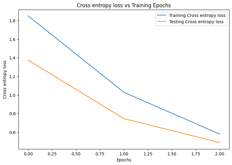 

\

\

plot_metrics(train_accs, test_accs, "Accuracy")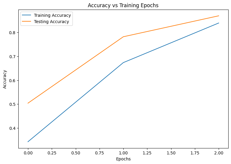 

\

Saving your model

The integration of tf.saved_model and DTensor is still under development. As of TensorFlow 2.9.0, tf.saved_model only accepts DTensor models with fully replicated variables. As a workaround, you can convert a DTensor model to a fully replicated one by reloading a checkpoint. However, after a model is saved, all DTensor annotations are lost and the saved signatures can only be used with regular Tensors. This tutorial will be updated to showcase the integration once it is solidified.

Conclusion

This notebook provided an overview of distributed training with DTensor and the TensorFlow Core APIs. Here are a few more tips that may help:

• The TensorFlow Core APIs can be used to build highly-configurable machine learning workflows with support for distributed training.
• The DTensor concepts guide and Distributed training with DTensors tutorial contain the most up-to-date information about DTensor and its integrations.

For more examples of using the TensorFlow Core APIs, check out the guide. If you want to learn more about loading and preparing data, see the tutorials on image data loading or CSV data loading.

\n

\ \

:::info Originally published on the TensorFlow website, this article appears here under a new headline and is licensed under CC BY 4.0. Code samples shared under the Apache 2.0 License.

:::

\